GTI Spreadsheet Top Tips: VLOOKUP

The markets are getting jittery, and what has worked in the recent past may not be the best thing to own going forwards. Global Trends Investor was designed to help you perceive and understand such changes in real time.

This is an explainer on how to get the most out of the Global Trends data spreadsheets we offer. It covers:

• The best way to track your own portfolio / watchlists each week
• How to set up a “VLOOKUP” formula in Excel
• Why it’s so powerful

The free GTI 200 spreadsheet and paid GTI Premium spreadsheet (2,500 stocks) are delivered to clients in Excel format.

One main use is naturally for analysing your own portfolio or other watchlists you may have.

The best way to do this is with a VLOOKUP function on Excel, which can allow you to simply and easily update CAPR scores and trend data for all stocks of interest every Monday.

So today, we’re going to walk through how that works.

Filtering To Your Portfolio

This is how the Leading Trends tab in the spreadsheet looks when you open it.

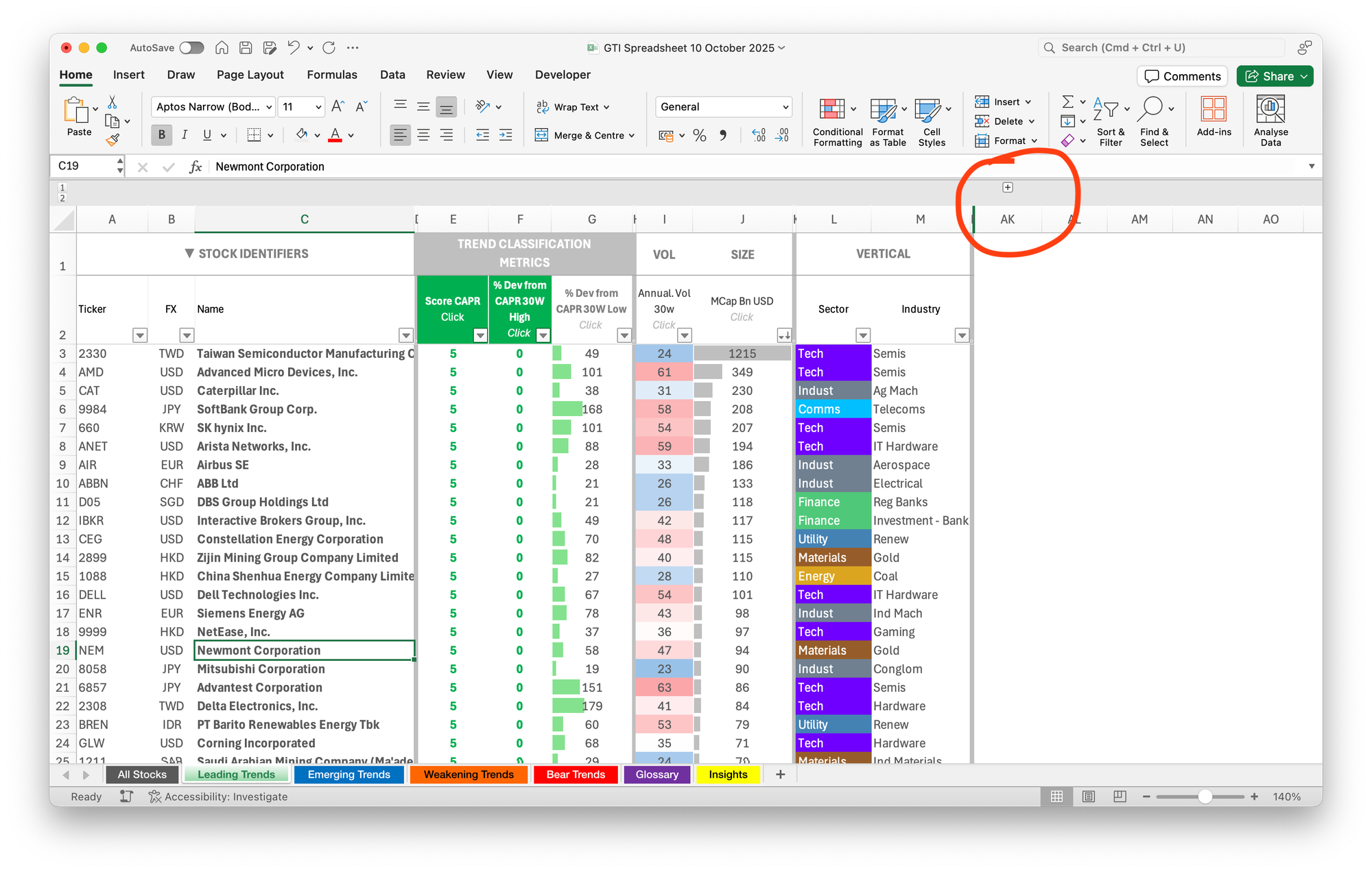
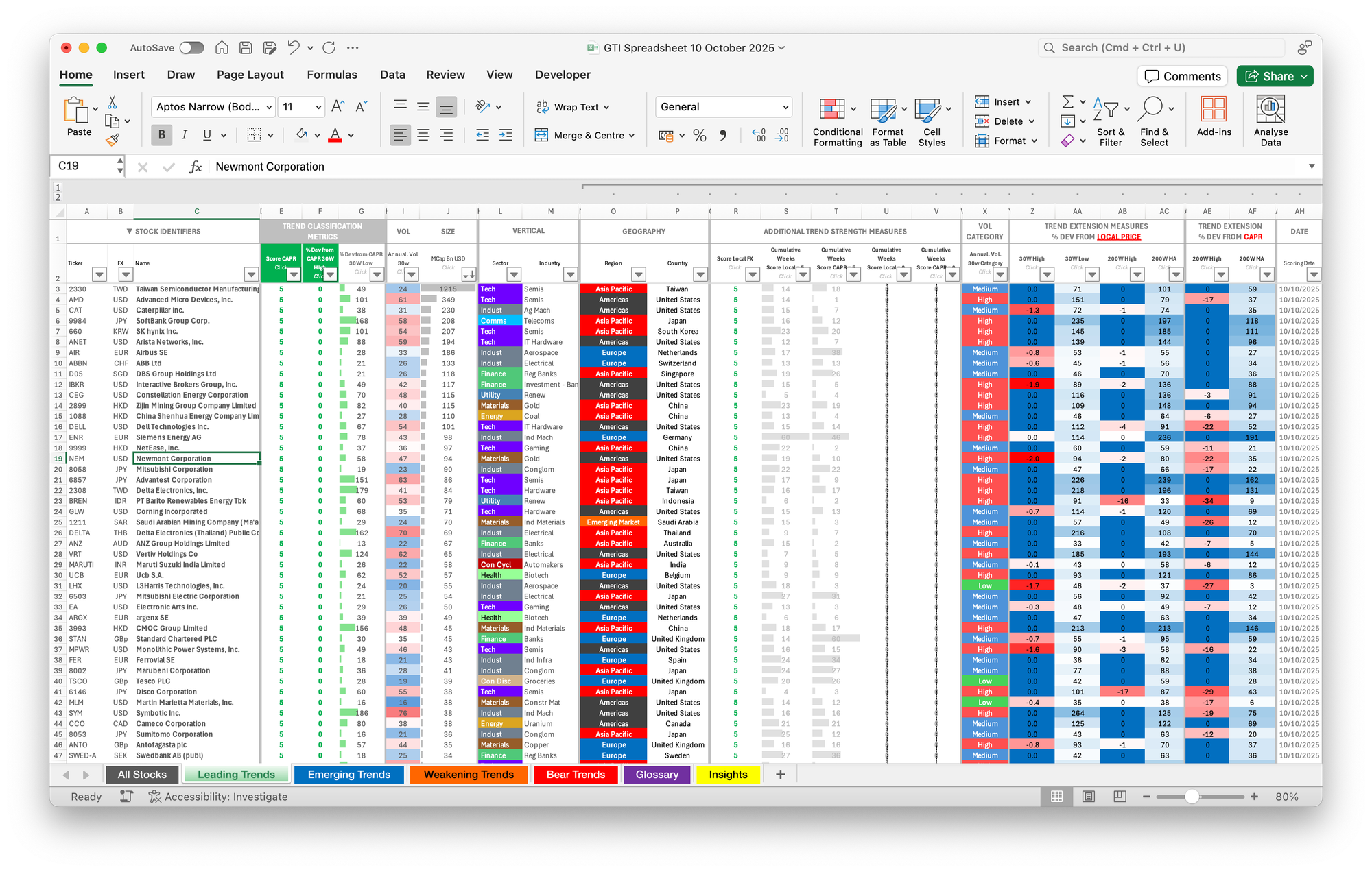
Hitting the little “plus” sign in the top bar (circled in red) will unpack another large set of trend data. This includes our measurements of trend time (how long a stock has been a 5 or a 0), and trend extension measures (how far they are from CAPR and price moving averages).

It will be tricky to see the details, but ultimately, the sheet looks like this:

So how do we use all this data to help analyse our own portfolio, or a list of new stocks?

One way is with Excel’s “VLOOKUP” feature.

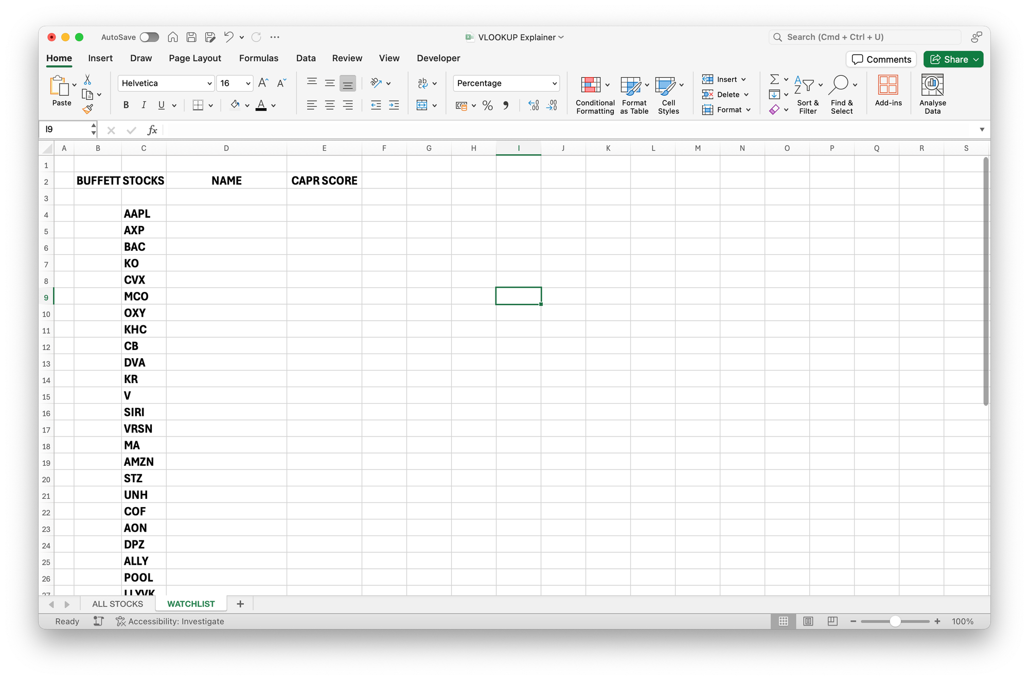
Step 1 is to load up the list of stocks you want to monitor. For example, here, we have dropped in Berkshire Hathaway’s list of current holdings.

Then you want to build in a feature that pulls in the data you want next to your list of tickers, from another sheet. That other sheet is where you can drop the “All Stocks” data each week, which will then automatically update the trend data for your specific watchlist.

This way, you can very quickly see how your portfolio or watchlist is doing when it comes to momentum.

The formula is called a “VLOOKUP”, and it works like this...

You can look for the ticker “AAPL” in a different tab, and then pull other data related to it from neighbouring cells. So next to AAPL, we could pull in its full name: Apple Inc.

The formula, as always, starts with an equals sign, "=".

Then you type in "VLOOKUP(", to get "=VLOOKUP(" as the base of the formula.

Then you have to make four choices:

1. The cell you want to match (AAPL),
2. The array of cells you want it to look for additional data in,
3. The number of columns across from the left you want the data from,
4. Whether it needs to be an exact match.

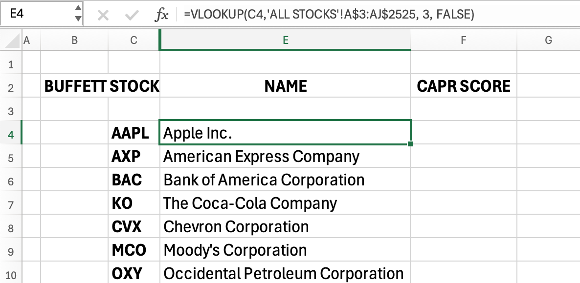
The formula, in this case, looks like this:

=VLOOKUP(C4,'ALL STOCKS'!A$3:AJ$2525, 3, FALSE)

Each category is separated by a comma, and in order, reflects these things:

• We want to find the content of cell C4 (“AAPL”),
• We want to find it in the 'All Stocks' tab in the A$3:AJ$2525 array of cells,
• We want to display what is 3 columns from the left,
• We want an exact match, so write “false”.

A couple of points to clarify. Firstly, the dollar signs in the second category are to fix the array to those cells, otherwise, when you copy the formula down the list, the array it looks in would also drop down by one cell each time, and you would get an error.

Secondly, the column number in the third category is always counted from the left, so for column C it’s 3, for E, it would be 5.

As always with Excel, you have to follow their rules, and write the formula perfectly or it won't work. There are other tutorials online if you get stuck, and AI is very helpful at troubleshooting too.

The result is here. You can see that the cell contains the formula, but displays the stock name. It has successfully pulled "Apple Inc." from the All Stocks tab, 3 columns into the array from the left:

As you see, having entered the formula into row 4, for AAPL, you can then copy it down to the rest of the list, which will auto-populate. The dollar signs in the formula are important, or copying it down won’t work.

Next, we want to repeat the exercise for the CAPR Score column.

In this case the formula will be:

=VLOOKUP(C4, 'ALL STOCKS'!A$3:AJ$2525, 5, FALSE)

It uses column 5, because that is column E in the All Stocks tab.

The result looks like this once the formula has been setup and copied down the list:

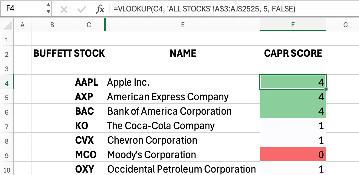
(The colours are added using “conditional formatting”)

When applying it to our own strategies and stock universes, we often use the sort and filter buttons, so that we can reorder the list by trend strength, and easily see which groups are strong and which are weak.

We also often use the trend time feature, to filter for new strong trends - companies which have just become a 5 for the first time. We can also do this for new weak trends (score of 0).

The final result is here:

And the best bit is yet to come.

Because now, when the GTI spreadsheet hits your inbox the following week, around 7.30am, you can very simply drop the All Stocks tab from GTI Premium (or the free GTI 200 spreadsheet) into your own ALL STOCKS tab. When you do, your watchlist or portfolio sheet will automatically update with the new week's scores.

Set it up once, and you can use it forever.

Naturally, you can also add VLOOKUPs for whichever columns you want to. You could do it for the whole thing if you liked, and it could look something like this:

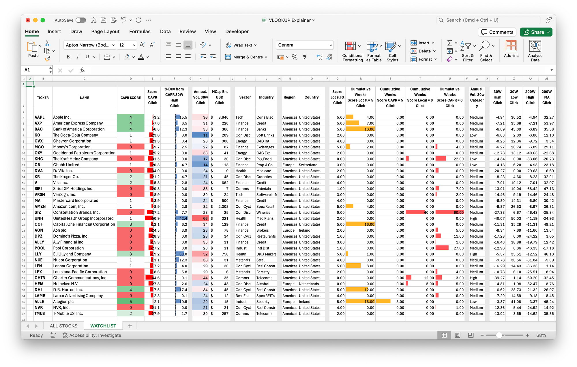
Having set it up once, it’s reasonably easy to copy the system over into another tab for a new watchlist or portfolio.

So there you have it. That's how you can use the "VLOOKUP" formula to build your watchlists and portfolios in Excel, to get the most out of our powerful Global Trends data.

This is a system that we use internally to keep track of the momentum of different strategies, our own and others. Remember, momentum is a valuable addition to any strategy – value, quality, growth, large caps or low vol stocks, in America, the UK, or Japan.

It’s an enhancement to whatever strategy you use.

Once set up, it can tell you in seconds what’s working and what’s not. For example, it’s notable that Berkshire Hathaway itself is a CAPR 1, as its portfolio of around 40 stocks only contains only one CAPR 5 in it – Allegion (ALLE). Until this week, quality has been underperforming this speculative bull market.

VLOOKUP Explainer Spreadsheet Download

We hope that’s been helpful.

Please go away and give it a go on the full sheet if you are a Premium client, or on the free GTI 200 spreadsheet if not.

Here is the one we built to help visualise this demonstration:

Feel free to download and use it as you wish.

If you have any questions or need additional clarifications on using Vlookups or the spreadsheet, please do let us know at gti@bytetree.com, as that will enable us to improve this guide for all clients.

All the best,

The Global Trends Team